Top 7 Machine Learning Models Used in Clean Energy Forecasting

Introduction

Imagine a future where solar panels and wind turbines adjust themselves in real time—maximizing power output based on evolving weather patterns, energy prices, and grid conditions. Picture entire cities tapping into renewable resources so efficiently that they rarely rely on fossil fuels. Or envision a farm that knows precisely when the sun will peak, allowing battery systems to store energy in anticipation of evening usage. This isn’t science fiction. These scenarios are rapidly coming to life thanks to machine learning models that drive clean energy forecasting.

Welcome to this comprehensive guide on how machine learning revolutionizes clean energy forecasting. In the quest to reduce carbon footprints, keep the grid stable, and lower operational costs, governments, utilities, and private enterprises are turning to advanced artificial intelligence (AI) solutions. Machine learning models form the backbone of these innovations: they interpret enormous streams of data—like weather forecasts, satellite imagery, historical consumption logs, and more—to deliver accurate, actionable predictions.

In this long-form post, our mission is to demystify the top 7 machine learning models commonly used for clean energy forecasting. You’ll discover:

1. A brief overview of why machine learning is vital to the clean energy revolution.
2. Deep dives into each of the seven models: how they work, when to use them, and real-world success stories.
3. A step-by-step implementation framework to get you started or accelerate your current projects.
4. Pro tips on optimizing these models and pitfalls to watch out for.
5. Answers to frequently asked questions about AI-driven energy forecasting—spanning from data requirements to ROI and regulation.
6. Opportunities for AdSense monetization and affiliate marketing partnerships, especially if you manage content platforms focusing on AI, data science, or sustainability.

By the end, you’ll possess the know-how to either select the right machine learning approach for your next clean energy project or refine an existing one for better outcomes. So grab your favorite beverage and prepare for a thorough exploration that merges data-driven intelligence with the world’s urgent need for renewable power.

Table of Contents

1. Clean Energy Forecasting 101
2. Why Machine Learning is Transforming Renewable Energy
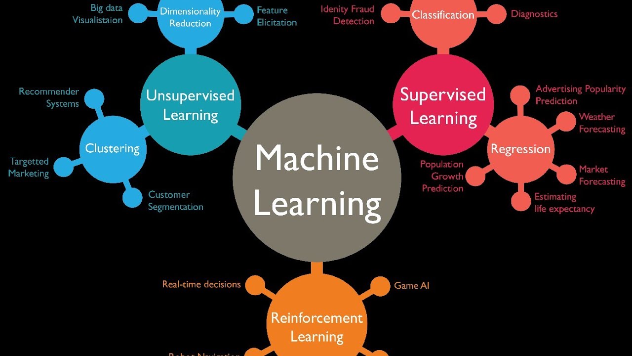
3. An Overview of the 7 Machine Learning Models
4. Model 1: Linear and Polynomial Regression
5. Model 2: ARIMA, SARIMA, and Time Series Approaches
6. Model 3: Decision Trees and Random Forests
7. Model 4: Gradient Boosting (XGBoost, LightGBM, CatBoost)
8. Model 5: Artificial Neural Networks (ANNs)
9. Model 6: Convolutional Neural Networks (CNNs) for Spatiotemporal Data
10. Model 7: Recurrent Neural Networks (RNNs, LSTMs, and GRUs)
11. Step-by-Step Blueprint for Implementing ML in Clean Energy Forecasting
12. Real-World Use Cases
13. Common Pitfalls and How to Avoid Them
14. FAQs
15. Conclusion

 

1. Clean Energy Forecasting 101

1.1 The Importance of Accurate Forecasts

Clean energy sources—like solar, wind, and hydro—are inherently variable. The sun doesn’t always shine, and wind speeds fluctuate drastically. Balancing power supply and demand requires accurate forecasts of how much energy can be produced when and where. This is essential for:

• Grid Stability: Utility operators must keep the lights on, adjusting for real-time load shifts.
• Financial Planning: Energy traders and asset managers need to price electricity correctly, factoring in expected generation.
• Storage Optimization: Batteries, pumped hydro, or hydrogen systems depend on forecasts to decide when to store energy or release it.

1.2 Data Sources in Clean Energy Forecasting

Before we jump to models, it’s crucial to note the data that fuels them:

1. Weather Data: Satellite images, ground station logs, atmospheric modeling from agencies like NOAA or ECMWF.
2. Historical Generation Records: Past performance of wind turbines or solar farms under varied conditions.
3. Location-Specific Metadata: Altitude, terrain features, shading from surrounding infrastructure.
4. Temporal Factors: Seasonal patterns, daily load cycles, local events or holiday schedules.

Machine learning thrives when it’s fed with robust, high-quality data. The synergy between advanced data sources and new-age ML techniques amplifies the reliability of clean energy forecasts—ultimately driving more stable, sustainable power grids.

2. Why Machine Learning is Transforming Renewable Energy

2.1 AI as a Game-Changer

Traditional forecasting methods—like persistence models (assuming tomorrow’s production is the same as today’s) or simple statistical approaches—often struggle with the complexity of real-world renewable energy. In contrast, machine learning excels at uncovering hidden relationships and quickly adapting to new data. This adaptability is priceless in an industry shaped by microclimates, evolving technologies, and uncertain policy frameworks.

2.2 Benefits of ML-Driven Forecasts

• Increased Accuracy: ML can reduce the margin of error in short-term and long-term predictions.
• Operational Efficiency: Plant operators can schedule maintenance or deployment times more effectively, slashing downtime.
• Economic Gains: Better forecasts reduce the need for expensive reserve power or real-time market corrections.
• Sustainability: AI-driven strategies can cut carbon emissions, as the grid runs more smoothly on renewables without frequent ramp-up of gas or coal plants.

2.3 Growing Demand from Stakeholders

From utility giants to small solar farm operators, the industry is hungry for predictive solutions that integrate easily and deliver quantifiable results. This appetite fuels investment in AI-based tools, with entire software platforms dedicated to optimizing wind farm output, scheduling solar farm expansions, or balancing microgrid resources in real time. If you’re considering diving into clean energy forecasting, there’s never been a better moment to harness the power of ML.

3. An Overview of the 7 Machine Learning Models

Let’s preview the 7 ML models we’ll explore in detail:

1. Linear and Polynomial Regression: The classic approach for basic relationships.
2. ARIMA, SARIMA, and Time Series Approaches: Tailored for cyclical data and trends over time.
3. Decision Trees and Random Forests: Interpretable, robust models for capturing non-linearities.
4. Gradient Boosting (e.g., XGBoost, LightGBM, CatBoost): State-of-the-art ensemble methods for improved accuracy.
5. Artificial Neural Networks (ANNs): The foundation of deep learning, capable of modeling complex patterns.
6. Convolutional Neural Networks (CNNs) for Spatiotemporal Data: Useful when dealing with images or geographical data.
7. Recurrent Neural Networks (RNNs, LSTMs, GRUs): Specialized in sequential data, which is crucial for time-based forecasting.

Why highlight these? Because each approach brings unique strengths and trade-offs—from interpretability to computational cost. Knowing which to apply can spell the difference between an acceptable forecast and a game-changing one.

4. Model 1: Linear and Polynomial Regression

4.1 Core Concept

Linear regression is among the simplest machine learning techniques: it tries to fit a line (or plane, in multiple dimensions) that minimizes the sum of squared errors between predicted and actual values. For clean energy, it might look like:

Power Output=β0+β1(Solar Irradiance)+β2(Wind Speed)+…\text{Power Output} = \beta_0 + \beta_1(\text{Solar Irradiance}) + \beta_2(\text{Wind Speed}) + \dots

However, real-world relationships can be more non-linear. Hence, we often use polynomial regression—extending the model with squared or cubic terms to capture curved patterns.

4.2 Use Cases in Clean Energy

• Initial Feasibility Studies: Quick checks on how a single factor (like wind speed) might correlate with turbine output.
• Small-Scale Facilities: Where data volume is limited, linear or polynomial regression can suffice, providing easy interpretability.
• Proof-of-Concept: Startups often begin with linear models to gauge whether more advanced techniques are warranted.

4.3 Pros and Cons

• Pros: Easy to implement; interpretable coefficients; minimal computational cost.
• Cons: May struggle with multi-dimensional or highly non-linear phenomena typical in solar or wind forecasting; can be outperformed by ensemble or deep models.

4.4 Implementation Tips

1. Data Normalization: Standardize or normalize your features if they vary widely (e.g., combining wind speeds in m/s with temperatures in °C).
2. Feature Engineering: For polynomial regression, carefully choose polynomial degrees—excessive degrees can cause overfitting.
3. Regularization: Use Ridge or Lasso to keep the model from going haywire with too many polynomial features.

5. Model 2: ARIMA, SARIMA, and Time Series Approaches

5.1 What is Time Series Forecasting?

Time series methods like ARIMA (AutoRegressive Integrated Moving Average) and SARIMA (Seasonal ARIMA) revolve around the concept that past values and patterns can predict future outcomes. They focus heavily on temporal correlations, a prime feature in clean energy data—where daily, weekly, or seasonal cycles matter.

5.2 ARIMA and SARIMA Breakdown

• ARIMA(p, d, q): “p” stands for the number of autoregressive terms, “d” for degree of differencing, and “q” for moving-average terms.
• SARIMA(p, d, q)(P, D, Q)_m: Extends ARIMA to handle seasonality with additional parameters “P, D, Q” for the seasonal part, and “m” indicating the length of the season (e.g., 24 for hourly cycles in a day).

5.3 Relevance to Clean Energy

1. Seasonal Solar Patterns: Solar irradiance shows daily periodicity. SARIMA can model the morning ramp-up and evening drop-off, plus longer seasonal trends.
2. Weekly Demand Cycles: Consumer demand for electricity might spike on weekdays or weekends, which can be integrated into a time series approach.
3. Long-Term Drifts: ARIMA can handle slow, consistent changes in wind patterns or grid usage.

5.4 Best Practices

• Stationarity Check: Use techniques like the Augmented Dickey-Fuller (ADF) test or differencing to achieve stationarity.
• Grid Search: Automated parameter search (like pmdarima in Python) can simplify the process of finding the best p, d, q values.
• Incorporate Exogenous Variables: ARIMAX or SARIMAX allows adding external features—like temperature or local events—to further refine your forecasts.

6. Model 3: Decision Trees and Random Forests

6.1 Introduction to Decision Trees

A decision tree splits your dataset based on certain features (e.g., wind speed < 5 m/s vs. wind speed ≥ 5 m/s) to minimize impurities in leaf nodes. It’s conceptually straightforward—like a flowchart for predictions—but can become unstable or overfit if grown too deep.

6.2 Random Forest

Random Forest—an ensemble of multiple decision trees—addresses single-tree weaknesses by averaging predictions from many slightly different trees. This typically yields better generalization and performance.

6.3 Utility in Clean Energy Forecasting

• Non-Linear Interactions: Trees handle complex relationships between variables, like when wind turbines’ power output saturates after a certain wind speed.
• Interpretability: Feature importance metrics show which factors heavily influence your forecast.
• Handling Mixed Data Types: Trees easily manage categorical variables (like region) alongside continuous ones (like humidity).

6.4 Example: Wind Power Prediction

Imagine you have data on wind speeds, direction, air density, and historical turbine production. A random forest can learn thresholds—like “If wind speed is between 3–15 m/s, output changes linearly, but beyond 15 m/s, output saturates.” This is simpler to interpret than black-box neural networks.

7. Model 4: Gradient Boosting (XGBoost, LightGBM, CatBoost)

7.1 The Power of Boosting

Gradient boosting builds models in a stage-wise fashion: each new tree tries to correct errors made by the previous ensemble. Over time, the ensemble converges toward better predictions. Popular frameworks—XGBoost, LightGBM, and CatBoost—have become staples in data science competitions due to their high accuracy and speed.

7.2 Why It Excels in Clean Energy

• Handles Large Datasets Efficiently: Energy systems can generate gigabytes of logs daily.
• Sparse Data Capability: CatBoost, for instance, gracefully handles categorical features, which might appear in location or equipment IDs.
• Hyperparameter Tuning: Tools like grid or Bayesian search can optimize parameters (e.g., learning rate, max depth) for maximum accuracy.

7.3 Use Cases

1. Short-Term Solar Forecasts: Predicting next-hour output based on real-time irradiance, temperature, and historical signals.
2. Hybrid Models: Combined with time series features (like lag variables), gradient boosting can outperform pure ARIMA on certain tasks.
3. Energy Price Forecasting: In deregulated markets, anticipating power prices helps schedule when to sell solar or wind output.

7.4 Implementation Notes

• Feature Engineering: Adding polynomial or lagged features can significantly boost performance.
• Regularization: Adjust gamma or lambda to prevent overfitting—critical in noisy datasets.
• Early Stopping: Minimizes overtraining by halting the boosting rounds when validation scores stop improving.

8. Model 5: Artificial Neural Networks (ANNs)

8.1 Fundamentals of ANNs

At their core, ANNs stack layers of artificial neurons, each applying linear transforms and non-linear activations to incoming data. The idea is to automatically learn hierarchical feature representations—something that can be gold for complex, multi-dimensional data often found in clean energy analysis.

8.2 Architectures for Energy Forecasting

1. Feedforward ANNs: Basic multi-layer perceptrons (MLPs) for simpler patterns.
2. Deep Networks: Multiple hidden layers capture more intricate relationships, like interactions between humidity, pressure, wind speed, etc.
3. Autoencoders: For dimensionality reduction or anomaly detection in sensor arrays.

8.3 Practical Case: Solar Farm Efficiency

A neural network can process data from:

• Satellite Cloud Imagery
• Ground-Level Observations
• Panel Age and Maintenance Logs

By learning correlations, it can predict the day-ahead or hour-ahead solar output, factoring in subtle cues like partial cloud cover or microclimate anomalies.

8.4 Limitations and Considerations

• Data-Hungry: Deep ANNs need large, diverse training sets.
• Black-Box: Harder to interpret than linear or tree-based methods. Some interpretability frameworks exist, but it’s still more opaque.
• Computational Cost: Training can be resource-intensive. Plan for GPU/TPU usage if your dataset is massive.

9. Model 6: Convolutional Neural Networks (CNNs) for Spatiotemporal Data

9.1 Why CNNs?

While CNNs emerged for image recognition, they also shine in tasks that involve spatial data—like weather maps or satellite imagery for cloud cover. Each CNN layer detects spatial features, from edges to complex shapes.

9.2 Spatiotemporal Forecasting in Clean Energy

Spatiotemporal means you track both space (geographical distribution of wind or clouds) and time (how it changes hour by hour). CNNs can interpret:

• Satellite Cloud Movement: Identify cloud patterns that might reduce solar output in 2 hours.
• Regional Wind Patterns: Model how a storm front moves across multiple wind farms.
• Sea Surface Temperatures: Predicting wave or tidal energy availability.

9.3 Implementation Overview

• Data Collection: Obtain satellite or radar data in the form of frames or sequences.
• Preprocessing: Convert images into consistent resolution, label each with corresponding energy outputs or meteorological variables.
• Model Architecture: Possibly combine CNN with RNN (for time dimension) or 3D CNNs that handle spatiotemporal input.
• Inference: The CNN “sees” the next 2–3 frames of weather patterns, predicting near-future solar/wind intensities.

10. Model 7: Recurrent Neural Networks (RNNs, LSTMs, and GRUs)

10.1 The Time-Sequence Edge

Standard neural networks assume independent data points, but RNNs track information across sequences. For long sequences, an RNN might face “vanishing gradients.” Solutions like LSTM (Long Short-Term Memory) and GRU (Gated Recurrent Unit) overcame this by introducing gating mechanisms that preserve memory over extended time steps.

10.2 Applications in Clean Energy

• Wind Power: An RNN or LSTM can handle daily or even sub-hourly sequences of wind data, capturing temporal patterns missed by simpler methods.
• Load Forecasting: Predicting how city-wide electricity demand might spike or drop in response to changing conditions.
• Multi-Step Forecast: RNN-based models can predict not just the next hour but also subsequent hours or days if properly trained.

10.3 Architectural Considerations

• Input Features: Often merges time series data with external signals (like temperature or day of week).
• Attention Mechanisms: In advanced setups, attention layers highlight crucial time steps.
• Dropout: Regularize the network to avoid overfitting on seasonal quirks.

10.4 Example: Tidal Energy Management

Tidal currents follow predictable lunar cycles but are also influenced by short-term weather. A well-tuned LSTM might incorporate both cyclical knowledge and real-time wave sensor data for high-precision forecasting—guiding whether it’s beneficial to store or dispatch power to the grid.

11. Step-by-Step Blueprint for Implementing ML in Clean Energy Forecasting

Now that you’ve learned about the top 7 models, let’s outline a robust implementation roadmap. This blueprint helps ensure you move from concept to production effectively—minimizing confusion and boosting ROI.

11.1 Step 1: Define Goals and Scope

• What’s the forecasting horizon? Hours, days, or weeks ahead?
• Which energy source(s)? Solar, wind, hydro, or a combination.
• Metric of success? Mean Absolute Error (MAE), Root Mean Squared Error (RMSE), or a cost-based measure?

11.2 Step 2: Gather and Clean Data

• Data Pipelines: Connect to weather APIs, SCADA logs, or satellite feeds.
• Data Quality: Check for missing or inconsistent records.
• Feature Engineering: Create lag features (e.g., wind speed from the last 6 hours), polynomial transformations, or domain-specific indicators (e.g., day length for solar).

11.3 Step 3: Model Selection and Prototyping

• Baseline: Start with simpler models (e.g., linear or ARIMA) for a reference.
• Shortlist: Based on your data shape, choose 2–3 advanced models (like random forests, XGBoost, or LSTMs).
• Hyperparameter Tuning: Use cross-validation or grid/random search to optimize performance.

11.4 Step 4: Model Evaluation and Validation

• Train/Test Split: Keep your test set strictly out-of-sample.
• Temporal Validation: Consider rolling or expanding windows in time series contexts to reflect real-life forecasting scenarios.
• Performance Metrics: Evaluate RMSE, MAPE, or custom cost functions. You might also gauge peak error if you’re more concerned about extremes.

11.5 Step 5: Deployment and Monitoring

• Containerization: Docker or Kubernetes for scalable ML service deployment.
• Real-Time Inference: If sub-hourly forecasts are needed, design a pipeline that automatically ingests fresh data.
• Monitoring: Set up alerting if forecast error spikes, possibly retraining models weekly or monthly as conditions evolve.

11.6 Step 6: Optimization and Maintenance

• Model Retraining: Data drift can degrade performance; schedule periodic retrains or trigger them when errors exceed thresholds.
• Feature Updates: If new data sources become available—like upgraded sensors—incorporate them.
• Cost-Benefit Analysis: Evaluate if complexities like CNN or RNN are warranted. Sometimes advanced approaches yield diminishing returns relative to simpler methods.

12. Real-World Use Cases

12.1 Hybrid Wind-Solar Farm Forecasting

Context: A utility-scale farm in Texas merges wind turbines and solar panels. The main challenge is dealing with two intermittent resources.
Solution: They combine a CNN to interpret satellite cloud formations for solar predictions with an LSTM that tracks wind speed patterns. Weighted ensemble logic merges the two predictions.
Result: Forecast errors drop by 25%, enabling the farm to confidently bid more power into the real-time electricity market.

12.2 Microgrid Management in Remote Communities

Context: A microgrid in a Pacific island community uses solar and wind, plus battery storage. Communication is patchy, and storms can be abrupt.
Solution: A random forest model runs on an on-site server with limited connectivity. It forecasts the next few hours of generation and consumption, guiding battery charging/discharging.
Result: Diesel generator usage is cut in half, and the community gains 24/7 reliable power.

12.3 Wind Farm Wake Effect Analysis

Context: Large offshore wind farm with turbines arranged in rows. Turbines in the second or third row face reduced wind due to wake effects from the front row.
Solution: A gradient boosting approach integrated with fluid dynamics simulations to capture wake patterns. It refines power forecasts for turbines downwind.
Result: Maintenance scheduling becomes more accurate, and the operator sees a 10% increase in annual net production.

13. Common Pitfalls and How to Avoid Them

1. Ignoring Physical Constraints
   • Issue: A model might predict negative power or exceed a turbine’s rated capacity.
   • Solution: Clamp outputs or integrate domain knowledge (like max turbine capacity) into the model.
2. Overfitting
   • Issue: With so many features and complex networks, it’s easy to produce a “perfect” solution for training data but fail in real-world usage.
   • Solution: Cross-validate thoroughly, apply regularization, and watch for large differences between training and test errors.
3. Not Considering Data Shifts
   • Issue: Weather patterns can shift over years, or new equipment changes relationships.
   • Solution: Implement continuous learning or a schedule for model updates to remain relevant.
4. Insufficient Domain Expertise
   • Issue: A purely data-driven approach might ignore meteorological realities or grid constraints.
   • Solution: Collaborate with meteorologists, engineers, or seasoned energy experts.
5. Technical Debt in Deployment
   • Issue: ML code might be messy, lacking versioning or rollback.
   • Solution: Embrace MLOps best practices—Dockerization, CI/CD pipelines, environment management.

Read Also: Decoding Blockchain’s Role in the Renewable Energy Market

FAQs

FAQ 1: Can small-scale renewable projects benefit from advanced ML models?

Absolutely. Even a small solar farm or single wind turbine can leverage random forests or basic neural networks to refine short-term forecasts. Cloud-based solutions reduce the need for on-site hardware.

FAQ 2: Which model should I start with if I’m new to ML?

Linear or time series models (like SARIMA) offer a gentle learning curve and often yield decent results. As data complexity grows, consider ensemble or neural network approaches.

FAQ 3: How important is real-time data ingestion for these models?

Crucial if your forecast horizon is short (e.g., hourly). Real-time data ensures you capture the latest weather shifts or equipment statuses. For daily or weekly forecasts, batch updates may suffice.

FAQ 4: Are there open-source tools specialized in clean energy forecasting?

Yes. Libraries like OpenEI or projects from NREL (National Renewable Energy Laboratory) might contain specialized datasets and frameworks. Many standard ML libraries (TensorFlow, PyTorch, scikit-learn) can be adapted to clean energy tasks, too.

FAQ 5: How do I handle outliers, like sudden sensor malfunctions?

Data validation is key. Implement anomaly detection—like an autoencoder or a robust scaler—to filter out sensor glitches before training your model. Fine-tuned random forests and boosting algorithms can also handle some outliers gracefully.

FAQ 6: Do I need a supercomputer to train deep neural networks for energy forecasting?

Not necessarily. Modern cloud providers offer GPU or TPU instances on pay-as-you-go plans. For moderate datasets, even a local GPU workstation might suffice. HPC resources become more relevant for extremely large or complex models (e.g., spatiotemporal CNNs).

FAQ 7: What about regulatory issues in AI-driven energy forecasting?

Regulations vary by region. Some grid operators require transparency in forecasting methods. Document your approach thoroughly and be prepared to share model performance metrics or error rates with regulators if needed.

FAQ 8: How do I integrate affiliate marketing in the clean energy and ML space?

Consider review posts or tutorials that mention specific IoT sensor platforms, data analytics software, or specialized GPU hardware. Offer discounted sign-up codes (if available) from cloud hosting providers that run advanced ML workloads.

FAQ 9: Does predictive maintenance tie into these forecasting models?

Very much so. Forecasting extends to equipment performance. ML can detect patterns that hint at turbine gearbox wear or PV panel degradation. Merging predictive maintenance with energy forecasting yields an even more robust operational framework.

FAQ 10: Which programming languages or libraries are best for these tasks?

Python dominates, with libraries like pandas, NumPy, scikit-learn, TensorFlow, PyTorch, and XGBoost. R also offers strong time series packages (forecast, prophet). Ultimately, pick the environment that aligns with your team’s skill set and your operational needs.

Conclusion

Machine learning stands at the forefront of the clean energy transformation, providing the intelligence to interpret volatile weather, manage fluctuating demand, and orchestrate complex power systems. Forecasting—a once-manual, often imprecise science—has become a data-driven discipline where advanced models can capture the nuances of solar irradiance, wind gusts, and grid load in ways unimaginable a decade ago.

We explored:

• 7 distinct machine learning models—from the humble linear regression to advanced CNNs and RNNs.
• Why each approach matters in clean energy contexts, highlighting real-world use cases.
• A step-by-step blueprint for implementing ML solutions, ensuring you address data management, model choice, validation, and operational deployment.
• Potential pitfalls, plus tips to avoid them, from data integrity to the inherent complexities of time-varying climate conditions.

Armed with this knowledge, you can start or enhance your AI-driven clean energy initiatives—whether that’s refining solar farm output predictions, optimizing wind farm scheduling, or harnessing multi-layered neural networks for spatiotemporal analytics. And if you run a blog, consulting firm, or educational platform, you can tap monetization opportunities via AdSense ads, affiliate links to specialized data and AI providers, or premium content offerings.

Action Steps

1. Choose Your Model: Identify which of the 7 aligns best with your data volume, complexity, and forecast horizon.
2. Assemble Quality Data: Don’t cut corners. The best model fails with poor inputs.
3. Iterate: Start with a baseline, refine features, and test advanced architectures.
4. MLOps for Production: Integrate versioning, containerized deployments, and continuous monitoring to keep your forecasting service reliable.
5. Expand: Evaluate if additional data sources—like satellite imagery for CNNs—can boost accuracy further.

Smart forecasting is more than an academic exercise; it’s the strategic edge that can reduce costs, stabilize the grid, and accelerate the shift to a sustainable energy future. So, dive in. Whether you’re a data scientist, an energy planner, or a green tech entrepreneur, harnessing machine learning models for clean energy forecasting might just be the next big leap toward a greener, more innovative tomorrow.